Our chilled water piping guide sets out the constraints a branch size must satisfy: mandatory velocity bands, European pressure-drop practice, material and insulation decisions. It stops short of arithmetic. This page does the arithmetic — one cooling load, carried through every equation, to a branch diameter. Where a limit is needed, we link back rather than restate it.
The case: a 105 kW group of fan coils on a 40 m branch run, sized in IFANNova’s UPVC 806 range. Every substitution is shown, every constant sourced, and four places flagged where a number gets taken from the wrong row, temperature, or chapter.

Cooling load converts to volumetric flow through one thermodynamic statement, written the same way in both unit systems:
Q = ρ · q · c · θ
Q = cooling capacity, ρ = water density, q = volumetric flow rate, c = specific heat of water, θ = temperature difference, return minus supply (Aircondlounge, Chilled Water Flow Rate Calculation, IP & SI). In SI, Q is in kW, ρ = 997 kg/m³, q in m³/s, c = 4.187 kJ/kg·°C, θ in °C. In IP, Q is in Btu/h, ρ = 62.4 lb/ft³, q in ft³/h, c = 1.0 Btu/lb·°F, θ in °F (same source).
Rearranged for the quantity you want:
q = Q ÷ (ρ · c · θ)
The first place people take the wrong value. Those ρ and c figures are nominal room-temperature properties, not chilled-water-temperature properties. ρ = 997 kg/m³ and c = 4.187 kJ/kg·°C are the values published by our HVAC source, which states them without giving a reference temperature, and every SI number on this page is computed with them — but the branch in Step 2 runs at 6.7 °C supply, well below the room-temperature conditions those nominal values correspond to. We could not obtain primary thermophysical data for liquid water at 4–7 °C, so we do not substitute a corrected value: chilled-water-temperature values for ρ and c: Coming soon. Carry the caveat rather than a guessed number. It is an assumption you are making, not a fact you have verified, and it belongs on the calculation sheet as one — the same way the 16 °C viscosity reference is flagged in Step 5 and sensitivity-tested in Step 8.
Before using any equation on your own project, run it against a worked example from the source. Two are published, and both reproduce exactly:
| Check | SI example | IP example |
|---|---|---|
| Load | 2110 kW | 600 RT = 600 × 12 000 = 7 200 000 Btu/h |
| Supply / return | 6.7 °C / 12.2 °C | 44 °F / 54 °F |
| θ | 5.5 °C | 10 °F |
| Substitution | 2110 = 997 × q × 4.187 × (12.2 − 6.7) | 600 × 12 000 = 62.4 × q × 1 × (54 − 44) |
| Result | q = 0.0919 m³/s = 91.9 L/s | q = 11 538.46 ft³/h = 1439 gpm |
Both examples are from Aircondlounge, Chilled Water Flow Rate Calculation (IP & SI). We recomputed both independently and got 0.0919 m³/s and 1438.6 gpm — agreement to the published rounding. That check confirms the equation was transcribed correctly before you trust it with a project load.
Most US hydronic work never writes ρ and c explicitly. It uses:
BTU/hr = 500 × GPM × ΔT, rearranged as GPM = BTU/hr ÷ (500 × ΔT)
The 500 is not a magic number. It is 8.33 (density of water, lb per gallon) × 1 (specific heat of water, Btu/lb·°F) × 60 (minutes per hour) ≈ 500 (MEP Academy, How to Convert GPM to BTU/hr for Hydronic Systems) — the same ρ · c product, pre-multiplied into gallons and minutes.
The second place people take the wrong value. The derivation tells you when the constant stops being 500: the moment the fluid is no longer water. Add glycol and the specific heat term drops. Specific heat falls to about 0.98 at 20% glycol, ~0.94 at 30%, and ~0.90 at 40%, giving adjusted constants of 485 (light glycol), 470 (medium) and 450 (heavy) (MEP Academy).
What that does to our branch case, run four ways:
| Fluid | Constant | Flow for 358 275 Btu/h at ΔT 9.9 °F | Change vs water |
|---|---|---|---|
| Water | 500 | 72.4 gpm | — |
| Light glycol (~20%) | 485 | 74.6 gpm | +3.0% |
| Medium glycol (~30%) | 470 | 77.0 gpm | +6.4% |
| Heavy glycol (~40%) | 450 | 80.4 gpm | +11.0% |
Constants and specific-heat values from MEP Academy; the flow figures are our arithmetic on those constants. An 11% flow increase can move a branch across a velocity limit and, on a marginal selection, up a pipe size. A glycol loop sized with 500 is not conservative — it is under-flowed, and the coil will not make its duty. Keep the fluid in the calculation header of every sizing sheet.
Our case: a 105 kW fan coil group, supply 6.7 °C and return 12.2 °C, so θ = 5.5 °C. We use the same supply and return basis as the verified SI example above, so the flow arithmetic can be traced against a published case. These are not the UFC design values and are not offered as such: 6.7 °C sits inside the 5.6–7.2 °C supply band (42–45 °F per UFC 3-430-09, Table 2-1), while 12.2 °C sits just above the bottom of the 11.1–15.6 °C return band (52–60 °F, same table) — so the two sets of figures are consistent, not in conflict. Note that the Fahrenheit values are the ones UFC publishes; the metric equivalents are conversions, not separately specified design values, so quote the °F figures when you cite UFC. Your project’s design temperatures come from your own specification — the pillar page covers where those figures originate and why ASHRAE and CIBSE practice differ.
Substituting into q = Q ÷ (ρ · c · θ):
q = 105 ÷ (997 × 4.187 × 5.5) = 0.004573 m³/s = 4.573 L/s = 16.5 m³/h
Cross-checking in IP: 105 kW = 358 275 Btu/h (29.9 RT), and ΔT 5.5 °C = 9.9 °F, so GPM = 358 275 ÷ (500 × 9.9) = 72.4 gpm. Converting the SI answer directly gives 72.5 gpm. The two paths agree to 0.1 gpm — the closing check that both unit systems were handled correctly. Our arithmetic; equations per Aircondlounge and MEP Academy as cited.
The third place people take the wrong value. A 0.1 gpm discrepancy is rounding. A few percent is not — it usually means θ was converted as a temperature rather than a temperature difference. A 5.5 °C difference is 9.9 °F, not 41.9 °F. Running the °F→°C offset on a delta is the most common unit error in this calculation, and it is obvious only if you cross-check. Cross-check.
Velocity follows from continuity, V = q/A, with A = πD²/4 on the internal diameter. In gpm/inch units PPI gives V = 0.4085·Q/DI², where V is in ft/sec, Q in gpm, and DI = inside diameter in inches (PPI Handbook of PE Pipe, 2nd ed., Ch.6, Eq. 1-8). 0.4085 is the standard gpm-to-fps conversion and reproduces V = q/A correctly in our checks: at 72.4 gpm in a 3.764 in bore it returns 2.09 ft/sec, which is the 0.637 m/s computed in SI below.
The fourth place people take the wrong value, and the most expensive. Plastic pipe is specified by outside diameter and pressure class; the velocity and friction equations need inside diameter. On thick-walled pressure pipe those differ sharply. IFANNova’s UPVC 806 PN16 at Φ110 has a 7.2 mm wall (per our catalogue), so the bore is 110 − 2(7.2) = 95.6 mm. Sizing on 110 mm overstates flow area by 32% — (110/95.6)² = 1.32 — and, because velocity is inversely proportional to area at fixed flow, understates velocity by 25%: (95.6/110)² = 0.755. Note those are not the same percentage; a 32% area error is a 25% velocity error, not a 32% one. HDPE PN16 at Φ110 carries a 10 mm wall, giving a 90 mm bore (per our catalogue). Two pipes marked Φ110 present materially different bores, and the pressure class tells you which.
For our 4.573 L/s branch, on a Φ110 UPVC 806 bore of 95.6 mm:
A = π(0.0956)²/4 = 0.007178 m²
V = 0.004573 ÷ 0.007178 = 0.637 m/s
Velocity across candidate bores, at the same flow (our arithmetic):
| Bore | Flow area | Velocity | Note |
|---|---|---|---|
| 95.6 mm (Φ110 UPVC 806 PN16, 110×7.2, per our catalogue) | 0.007178 m² | 0.637 m/s | Largest bore we manufacture in pressure pipe |
| 66.0 mm | 0.003421 m² | 1.337 m/s | Illustrative bore |
| 55.4 mm | 0.002411 m² | 1.897 m/s | Illustrative bore |
| 44.2 mm | 0.001534 m² | 2.980 m/s | Illustrative bore |
Only the 95.6 mm row is a catalogue-verified IFANNova dimension. The other three are arithmetic illustrations of how sharply velocity climbs as area falls, not size offerings. The full UPVC 806 PN16 wall table is published across the range: 20×2.0, 25×2.0, 32×2.4, 40×3.0, 50×3.7, 63×4.7, 75×5.6, 90×6.7 and 110×7.2 mm (per our catalogue), so the bore for any size we sell is OD − 2×wall from that list. Take the exact bore from the dimension table for the size and pressure class you are buying.
Velocity roughly triples between the first and last row while the load never changes. That is why velocity is checked before pressure drop: it moves fastest, and the mandatory limits are written against it. Which limits apply, and the trap in reading the SI column of the ASHRAE 90.1 table, are covered in the pillar guide.
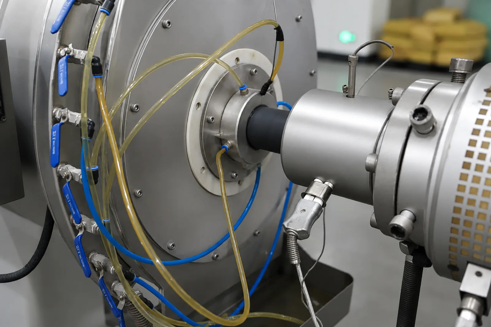
Two families are in service, and choosing between them is a real engineering decision rather than a preference.
ASHRAE Handbook—Fundamentals, Chapter 22 gives it in SI as Δp = f (L/D)(ρV²/2), with Δp in Pa, L and D in m, ρ in kg/m³ and V in m/s; and in head form Δh = f (L/D)(V²/2g), with Δh the energy loss in m and g the acceleration of gravity in m/s². The IP form carries a gc term of 32.2 ft·lbm/lbf·s², with Δp in lbf/ft², L and D in ft, ρ in lbm/ft³ and V in fps (ASHRAE Handbook—Fundamentals, Ch.22, IP and SI). PPI states the head form identically for PE: hf = f·(L/d’)·(V²/2g), with hf in ft of liquid, d’ = inside diameter in ft, g = 32.2 ft/sec², and f dimensionless but dependent on surface roughness and Reynolds number (PPI Handbook of PE Pipe, 2nd ed., Ch.6, Eq. 1-7).
The pressure form and the head form are the same equation — Δp in Pa, Δh in metres of fluid. Reporting a head-form answer as pressure is a factor-of-ρg error, about 9777 in SI (997 × 9.807). If a friction result looks off by three orders of magnitude, this is why.
ASHRAE Ch.22 also carries Hazen-Williams, in SI as Δp = 10.67·(Q/C)1.852·(L/D4.87). In head-loss form the two unit systems are:
(Hazen–Williams equation reference; ASHRAE Ch.22 SI for the Δp form.) The method is empirical, intended for water in full pressurised pipes, and best suited to turbulent conditions. Read the unit lists twice — the US customary form takes gpm and inches, not ft³/s and feet, while the SI form takes base units throughout. The coefficients 10.67 and 10.44 exist to absorb those unit choices, so the forms are not interchangeable. A related trap: the widely reproduced 4.52 coefficient belongs to a different form again — it returns pressure gradient in psi per foot, not head in feet. ASHRAE also renders its numbered Hazen-Williams equations as images, so we could read the SI Δp form as text but not verify the IP form from the primary source — hence the separate citation for the head-loss forms.
This is where branch calculations quietly go out of scope. Hazen-Williams “assumes that the water contains no additives and is close to 60 °F (15.6 °C)”, applies to water only, and is less accurate “for larger pipes and higher flow velocities”. Its C factors were “measured at a velocity of 3 feet per second (fps)” (0.91 m/s). NFPA 750 requires Darcy-Weisbach “if fluid velocity exceeds 25 fps (7.6 m/s)”. Overall, “the Hazen-Williams formula comes within 10 percent accuracy of the value obtained using the Darcy-Weisbach equation” (ASPE Pipeline, Hazen-Williams and Darcy-Weisbach Equations: Similarities and Differences).
PPI states the temperature limitation more directly: “The Hazen-Williams formula for water at 60 °F (16 °C) can be applied to water and other liquids having the same kinematic viscosity of 1.130 centistokes… The viscosity of water varies with temperature, so some error can occur at temperatures other than 60 °F (16 °C)” (PPI Handbook of PE Pipe, Ch.6).
Read that against a chilled water loop. The reference is 16 °C; chilled water runs at 4–7 °C. Every Hazen-Williams chilled water calculation is therefore run below the temperature its C factors were calibrated at, on water that is more viscous than the reference. That does not disqualify the method. It is the reason to treat its answer as an approximation with a known direction of error, and to use Darcy-Weisbach when the number is load-bearing. Two further disqualifiers: glycol is not water, so a glycol loop is outside its stated scope entirely; and a branch above 7.6 m/s falls under the NFPA 750 requirement above.
Darcy-Weisbach needs f, and f depends on the flow regime. ASHRAE defines Reynolds number as Re = ρVD/μ = VD/ν, where μ = dynamic viscosity (Pa·s) and ν = kinematic viscosity (m²/s), Re being dimensionless (ASHRAE Handbook—Fundamentals, Ch.22, SI). PPI gives a gpm/inch form: Re = 3126·Q/(k·DI), with Q in gpm, k = kinematic viscosity in centistokes, and DI in inches (PPI Ch.6, Eq. 1-12). Note that the dimensionally exact coefficient for these units is 3163, so PPI’s printed 3126 runs about 1% low; the difference is immaterial to the flow regime it is used to identify.
Liquid flow “will assume one of three flow regimes… laminar, turbulent or in transition”. Below Re 2000 the flow is laminar, “the pipe’s surface roughness has no effect and is considered negligible”, and f = 64/Re. Above Re 4000 the flow is turbulent and f depends on both Reynolds number and surface roughness, from the Moody Diagram or the Colebrook formula (PPI Handbook of PE Pipe, Ch.6, Eq. 1-9, 1-10).
For our branch, using the 1.130 cSt reference viscosity (PPI, at 16 °C — see the Step 0 note):
Re = VD/ν = (0.637 × 0.0956) ÷ 1.130×10⁻⁶ = 53 900
Firmly turbulent, an order of magnitude above the 4000 threshold — the normal answer for building chilled water. Surface roughness is therefore in play, pipe material genuinely affects the result, and f cannot be read off the laminar formula. This bore would need velocity below about 0.047 m/s to reach transition, a condition you would never design for.
The Colebrook equation for the Darcy friction factor is:
1/√f = −2·log₁₀( ε/3.7D + 2.51/(Re·√f) )
where ε = absolute roughness of the pipe wall (m in SI, ft in IP), D = internal diameter, and Re = Reynolds number. It is implicit in f — f appears on both sides — and therefore requires iteration (ASHRAE Handbook—Fundamentals, Ch.22, SI).
“Requires iteration” is where most published examples stop. Here is the iteration, for our branch at Re = 53 900, D = 0.0956 m, ε = 0.0015 mm, starting from a guess of f = 0.020:
| Pass | f in | f out | Change |
|---|---|---|---|
| 1 | 0.020000 | 0.020681 | +3.4% |
| 2 | 0.020681 | 0.020596 | −0.41% |
| 3 | 0.020596 | 0.020606 | +0.05% |
| 4 | 0.020606 | 0.020605 | −0.005% |
| 5 | 0.020605 | 0.020605 | converged |
Our computation, using the Colebrook form as published by ASHRAE Ch.22. Three passes gets you within 0.05%, far inside the uncertainty of everything else on the sheet. The starting guess barely matters — the equation is strongly self-correcting, which is why a hand solution is practical and why “it needs iteration” is not a reason to reach for Hazen-Williams instead.
ε is the one input where two defensible published conventions disagree. Picking one without knowing the other exists is a quiet source of mismatched calculations between design offices.
| Material / convention | Absolute roughness ε | Source |
|---|---|---|
| PE and other thermoplastics — US “smooth pipe” convention (same value as PVC/CPVC and drawn copper tubing) | 0.000005 ft = 0.0015 mm | PPI Handbook of PE Pipe, Ch.6 roughness table; SimuPipe, stated to follow Moody, Crane TP-410 and Colebrook |
| Thermoplastic pipe — German/European practice; HDPE per SimuPipe | k = 0.007 mm (0.000023 ft); 0.01 mm commonly used for PE as a conservative design value | KRAH, citing DVS 2210-1; SimuPipe |
| Commercial steel or wrought iron (new) | 0.00015 ft = 0.045 mm | PPI Ch.6 table; SimuPipe |
| Uncoated cast iron | 0.00085 ft | PPI Handbook of PE Pipe, Ch.6 |
PPI’s table carries the defining note: “Pipes that have absolute roughness equal to or less than 0.000005 feet are considered to exhibit ‘smooth pipe’ characteristics.” European nomograms built on Colebrook-White instead use k = 0.007 × 10⁻³ m per DVS 2210-1. Cite that last one with care: the DVS standard is paywalled and the attribution was verified through indexed page content rather than a full page load. SimuPipe also warns that “published ranges vary by source and pipe condition.”
Does the split matter? We ran our branch on all four values (our computation):
| ε used | f | Pressure gradient | Δp over 40 m | vs smooth |
|---|---|---|---|---|
| 0.0015 mm (US smooth-pipe) | 0.02060 | 43.6 Pa/m | 1744 Pa | — |
| 0.007 mm (DVS 2210-1 thermoplastic) | 0.02082 | 44.1 Pa/m | 1762 Pa | +1.0% |
| 0.01 mm (conservative PE) | 0.02093 | 44.3 Pa/m | 1772 Pa | +1.6% |
| 0.045 mm (new commercial steel) | 0.02219 | 47.0 Pa/m | 1878 Pa | +7.7% |
The honest answer for a branch at this Reynolds number: the US/European plastics convention split is worth about 1.6% and will never change a pipe size. Do not lose an afternoon to it. Plastic against new steel is worth 7.7% on friction — and against aged steel, considerably more, which is the next point.
Everything above treats ε as a constant. For plastic it approximately is. For metal it is not, and this is the part of a sizing calculation that is about year 20 rather than day one.
The Hazen-Williams C factor makes the effect legible. ASHRAE states: “C = roughness factor. Typical values of C are 150 for plastic pipe and copper tubing, 140 for new steel pipe, down to 100 and below for badly corroded or very rough pipe” (ASHRAE Handbook—Fundamentals, Ch.22, SI). PPI lists “C = Hazen-Williams Friction Factor, dimensionless, c = 150-155 for PE, (not related to Darcy-Weisbach friction factor, f)”, with its worked examples using C = 150 (PPI Ch.6). Heed that parenthesis: C is a roughness coefficient where higher means smoother, f a friction factor where higher means more loss. They are not convertible and never appear in the same equation.
PPI is explicit about the time dependence: “For water applications, HDPE pipe’s Hazen and Williams C factor for design is 150 and does not change over time. In contrast, the C factor for iron pipe and other traditional piping products declines dramatically over time due to corrosion and tuberculation or biological build-up” (PPI TN-27/2009).
The design consequence, stated as engineering judgement rather than a measured claim: a steel branch at C = 140 and a plastic branch at C = 150 look close on day one. If the steel line’s C drifts toward the 100 ASHRAE lists for badly corroded pipe, the friction term rises by about 86% at constant flow on the Hazen-Williams exponents — (140/100)1.852 = 1.86, since head loss scales as C−1.852 — while the plastic line, on PPI’s evidence, does not move. Whether you build that margin into the initial size or into the pump head is a project decision. Whether it exists is not.
A recurring objection to fused plastic pipe is that the internal weld bead adds resistance. PPI addressed it directly: “The fusion bead has very little effect on the flow as it is basically rounded and protrudes very little on the inside surface of the pipe. Secondly, the Hazen-Williams C-factor of 150 takes into account the inner bead… The Hazen-Williams Friction Factor, C, for PE pipe was determined in a hydraulics laboratory using heat fusion joined lengths of pipe with the inner bead present” (PPI TN-27/2009).
The load-bearing detail is the last clause: C = 150 was measured on fused pipe with the bead in place, not on a bead-free idealisation needing a penalty. Applying your own bead correction on top of C = 150 double-counts. Separately, IFANNova’s HDPE line uses the 603/604 compression fittings — no fusion, so the question does not arise (per our catalogue).
Every step together for the 105 kW branch on 40 m of Φ110 UPVC 806 PN16 (bore 95.6 mm, per our catalogue):
| Step | Equation | Substitution | Result |
|---|---|---|---|
| 1. Flow from load | q = Q/(ρ·c·θ) | 105 ÷ (997 × 4.187 × 5.5) | 0.004573 m³/s = 4.573 L/s |
| 2. IP cross-check | GPM = BTU/hr ÷ (500·ΔT) | 358 275 ÷ (500 × 9.9) | 72.4 gpm (vs 72.5 converted) |
| 3. Internal diameter | D = OD − 2·wall | 110 − 2(7.2) | 95.6 mm |
| 4. Area | A = πD²/4 | π(0.0956)²/4 | 0.007178 m² |
| 5. Velocity | V = q/A | 0.004573 ÷ 0.007178 | 0.637 m/s |
| 6. Reynolds | Re = VD/ν | (0.637 × 0.0956) ÷ 1.130×10⁻⁶ | 53 900 — turbulent |
| 7. Friction factor | Colebrook, iterated | ε = 0.0015 mm, 3 passes | f = 0.0206 |
| 8. Pressure drop | Δp = f(L/D)(ρV²/2) | 0.0206 × (40/0.0956) × (997 × 0.637²/2) | 1744 Pa over 40 m = 43.6 Pa/m |
Our arithmetic throughout, on the equations and constants cited above. Whether 0.637 m/s and 43.6 Pa/m are acceptable is a question for the velocity and pressure-drop limits in the pillar guide, where those bands and their sources live. This page establishes how you get to the two numbers you then check.
Run the same branch through Hazen-Williams at C = 150 (PPI’s design value for plastic):
hf = 10.67 × 40 × 0.0045731.852 ÷ (1501.852 × 0.09564.8704) = 0.1708 m of water over 40 m. Converting head to pressure gradient: 0.1708 × 9777 ÷ 40 = 41.7 Pa/m.
Against Darcy-Weisbach’s 43.6 Pa/m, Hazen-Williams comes in 4.3% low (41.7 vs 43.6). That sits inside ASPE’s stated expectation that “the Hazen-Williams formula comes within 10 percent accuracy of the value obtained using the Darcy-Weisbach equation” (ASPE Pipeline). Two independent methods agreeing to 4% is a genuine verification. Two methods disagreeing by 40% means a unit error somewhere, and the head-versus-pressure confusion in Step 4 is the usual culprit.
Our viscosity is the 16 °C reference value, not a chilled-water value we could source, so we ran the sensitivity: holding everything else fixed, raising ν by 30% moves the gradient to 46.2 Pa/m (+6.0%) and by 40% to 47.0 Pa/m (+7.8%) (our computation). Those are illustrative sensitivities, not a claim about the viscosity of water at 6 °C. The shape of the exposure is the point. Even a large viscosity error moves friction by single-digit percent, because f responds weakly to Re in this turbulent range, whereas velocity moved threefold across the diameters in Step 3. Get the bore and the flow right, and fluid-property uncertainty will not decide the size.
Once one size is solved, PPI gives a shortcut for the next: “When the friction loss through one size pipe is known, the friction loss through another pipe of different diameter may be found by” the diameter-ratio relation hf1 = hf2 × (d’1/d’2)5 (PPI Handbook of PE Pipe, Ch.6, Eq. 1-15), with the stated conditions that both pipes have the same surface roughness and the fluid the same viscosity and flow rate. PPI prints the exponent as 5; the Hazen-Williams diameter exponent is 4.87. Scaling our 95.6 mm result to 66.0 mm gives a factor of 6.08 on the Hazen-Williams exponent and 6.35 on PPI’s 5 — close enough that either supports the same engineering conclusion.
What that exponent means in practice is the most useful single fact in pipe sizing: friction goes as roughly the inverse fifth power of diameter. Our branch, at constant 4.573 L/s (our arithmetic, Darcy-Weisbach with ε = 0.0015 mm):
| Bore | Velocity | Re | f | Pressure gradient | vs 95.6 mm |
|---|---|---|---|---|---|
| 95.6 mm | 0.637 m/s | 53 900 | 0.02060 | 43.6 Pa/m | — |
| 66.0 mm | 1.337 m/s | 78 100 | 0.01906 | 257.2 Pa/m | 5.9× |
| 55.4 mm | 1.897 m/s | 93 000 | 0.01840 | 596.0 Pa/m | 13.7× |
| 44.2 mm | 2.980 m/s | 116 600 | 0.01763 | 1765.7 Pa/m | 40.5× |
Same load, same fluid, same 40 m. Dropping roughly one size band multiplies friction by about six; dropping to less than half the bore multiplies it by forty. A branch one size undersized does not cost a little pump energy — it costs a lot, permanently, and it cannot be commissioned out.
Note also that f actually falls as the pipe gets smaller, because Re rises. Anyone reasoning from the friction factor alone would conclude the small pipe is more efficient. The V² and 1/D terms dominate by an enormous margin. Never judge a size by f.
One correction, offered because it cost us real time and it is repeated across most of the pages that rank for this query.
The widely quoted hydronic sizing limits — 4 fps for pipe 2 in. and below, 4 ft of water per 100 ft above 2 in., the 0.75–10 ft/100 ft friction band, the 2–15 fps envelope and the erosion-velocity tables — are routinely attributed to ASHRAE Handbook—Fundamentals, Chapter 22. We opened both the IP and SI official pages for that chapter. They are not there. Chapter 22 covers the equations and the sizing procedure — Darcy-Weisbach, Colebrook, Reynolds number, Hazen-Williams and the C-factor prose, all cited above. It carries no prescriptive velocity limits.
Those limits most likely live in ASHRAE Handbook—HVAC Systems & Equipment, Chapter 13 (Hydronic Heating and Cooling), which is paywalled; every freely accessible copy returned HTTP 403 or no technical text. A secondary source does compile such limits — 2 in. and below at 4 fps (1.2 m/s), above 2 in. at 4 ft per 100 ft (400 Pa/m), a 2–15 fps envelope, plus Carrier-attributed figures by system section — crediting ASHRAE Fundamentals and the Carrier Pipe Design Manual (Aircondlounge, Chilled Water Pipe Sizing Guide). We could not confirm them in the chapter that source names, so treat them as secondary.
The practical instruction: if a vendor’s sizing chart cites “ASHRAE Fundamentals Chapter 22” for a velocity limit, the citation is wrong as given, whatever the merits of the number. Size against the mandatory limits your jurisdiction adopts — the pillar guide sets out which those are — not against a rule of thumb with a borrowed reference.
Worked arithmetic is only useful if it terminates in something orderable, so the limits of our supply belong in the same document as the equations.
IFANNova pressure pipe stops at Φ110: UPVC 806 PN16 and HDPE PN16 marked to DIN 8077/8078 (per our catalogue) both run Φ20–Φ110, and PPR PN20 exists only in 20, 25 and 32 mm (per our catalogue). If your calculation lands on a required bore above 95.6 mm, it has left our range and you need a mains supplier. PPR above 32 mm: Coming soon. Within the range, fitting depth decides a clean take-off: 203 UPVC fitting items including ball valves and solvent cement, 75 PPR items, the 603/604 HDPE compression series that needs no fusion plant, and brass 2405 fittings and valves for threaded transitions at 1/4 in – 1 in (per our catalogue).
What we will not publish is a diameter-versus-flow selection chart. A credible one is derived from licensed friction curves we cannot reproduce, and an invented one fails exactly where it matters. We have shown every equation those charts are built from instead, with sources named, so you can compute the number yourself and check anyone else’s chart against it.
Insulation can be supplied alongside the pipe; material, thickness and vapour barrier specification: Coming soon, advised per project. MOQ, lead time, pricing and certificate numbers: Coming soon. IFANNova is a French brand manufactured in our own facility by Zhuji Fengfan Piping Co., Ltd, Zhejiang, China — 30+ years, 1000+ employees, 118+ export countries, 120,000 m² (per our catalogue).
Should I use Hazen-Williams or Darcy-Weisbach for chilled water?
Darcy-Weisbach is the general one and the safer default. Hazen-Williams assumes water with no additives close to 60 °F (15.6 °C), applies to water only, loses accuracy for larger pipes and higher velocities, and its C factors were measured at 3 fps (0.91 m/s); NFPA 750 requires Darcy-Weisbach above 25 fps (7.6 m/s) (ASPE Pipeline). PPI notes the formula is calibrated to 1.130 centistokes at 60 °F (16 °C) and that “some error can occur at temperatures other than 60 °F” (PPI Ch.6). Chilled water at 4–7 °C sits below that reference, so Hazen-Williams is used outside its calibration temperature on every chilled water job. Expect agreement within about 10% (ASPE Pipeline); our branch case came out 4.3% apart.
Is the Hazen-Williams C the same as the Darcy friction factor f?
No, and PPI’s symbol list says so explicitly: “C = Hazen-Williams Friction Factor, dimensionless, c = 150-155 for PE, (not related to Darcy-Weisbach friction factor, f)” (PPI Ch.6). Higher C means smoother; higher f means more loss. They belong to different equations and are not convertible.
Why is my velocity higher than I calculated?
Almost always because the outside diameter was used instead of the bore. UPVC 806 PN16 at Φ110 has a 7.2 mm wall and therefore a 95.6 mm bore; HDPE PN16 at Φ110 has a 10 mm wall and a 90 mm bore (per our catalogue). Sizing Φ110 UPVC on 110 mm rather than 95.6 mm overstates flow area by 32%, which understates the velocity you will actually get by 25%.
How many Colebrook iterations are needed?
Three. On our branch case at Re = 53 900, starting from f = 0.020, the successive changes were +3.4%, −0.41%, +0.05% and −0.005% (our computation). The equation is self-correcting and the starting guess is close to irrelevant.
Do the ASHRAE velocity limits come from Fundamentals Chapter 22?
No. We opened both the IP and SI official pages of that chapter: it contains Darcy-Weisbach, Colebrook, Reynolds number and Hazen-Williams, and carries no prescriptive velocity limits. The commonly cited hydronic limits most likely sit in ASHRAE Handbook—HVAC Systems & Equipment, Chapter 13, which we could not access. Do not accept “ASHRAE Fundamentals Ch.22” as the source for a velocity limit.
What do I send you to get a branch quotation?
The required bore per size with quantities, the material, your specification’s design supply and return temperatures, and the total metres per size. If your computed bore exceeds 95.6 mm you are above our pressure-pipe ceiling of Φ110 and we will tell you so rather than waste a tender cycle (per our catalogue). Pricing, MOQ and lead time: Coming soon.
What one floor of chilled water branch pipework actually consumes: valve authority, strainer sizing, and the fitting counts that stop a site when they are missed.
Primary, primary-secondary and variable-flow chilled water loops compared — and which layer of the system a branch pipe supplier actually serves.
Expansion loops, anchors and guides for plastic chilled water pipe: how to size the offset leg, where to fix, and the engineering cost of choosing plastic.